Prometheus Metrics Types - A Deep Dive

Prometheus tracks four core metric types. Choosing the right one matters more than most developers realize. Pick the wrong type, and you’ll end up with slower queries, higher storage costs, or graphs that don’t reflect reality.

This guide explains each metric type clearly, including how it behaves, where it fits best, and which PromQL functions are compatible with it in production. The goal isn’t to cover theory, it’s to help you avoid mistakes that show up in real systems.

You’ll learn:

• When to use a counter, gauge, histogram, or summary, based on real-world usage
• How each type affects query performance and storage
• PromQL patterns for alerting, debugging, and dashboards

What Are Metrics in Prometheus?

In Prometheus, metrics are how you track what’s going on in your system, whether it’s the number of HTTP requests, CPU usage, or error rates. Each metric is made up of one or more time series, which means you’re recording how that data point changes over time.

A Prometheus metric includes:

• Metric name: Describes what’s being measured. Example: http_requests_total
• Labels: Key-value pairs that add detail. For instance: {method="POST", status="500"}
• Value: The actual measurement, like a count or gauge reading
• Timestamp: When the data was recorded (added automatically during scraping)

Here’s a practical example:

user_logins_total{user_type="admin", location="EU"} 193

This tells you that, at the time of the latest scrape, there were 193 logins by EU-based admin users.

Prometheus uses a pull model, meaning it scrapes metrics from your services at fixed intervals. This makes the system more robust; your app doesn’t have to push anything or worry about retries.

Every unique combination of metric name and labels becomes a distinct time series. This gives you detailed observability, but it also means you need to be careful. Too many label combinations can lead to high cardinality, which impacts performance and query speed.

High cardinality isn’t bad, but not every label adds value. Avoid dynamic values like user IDs or timestamps unless they serve a clear purpose. When detailed breakdowns are needed, make sure your backend can handle the load. Last9 is built for that.

Prometheus Metric Types

Each Prometheus metric type comes with trade-offs: how they store data, how they aggregate, and how they behave under real workloads.

• Use Counters when you need a reliable, ever-increasing total. Just remember they reset on process restarts, so use rate() or irate() to smooth that out in queries.
• Gauges are flexible but can be misleading if scraped at the wrong time. They’re great for current state, but not ideal for trends unless sampled consistently.
• Histograms give you a full view of value distributions, like how long requests take across buckets. They work well with aggregation but require tuning upfront: bad bucket design can make the data noisy or useless.
• Summaries are precise but isolated: they calculate quantiles locally and don’t merge well across instances. Use them when you care about accuracy on a single service, not across a fleet.

Quick Start: 30-Second Metric Selection

The 3 Cardinality Traps That Kill Prometheus

It’s easy to add labels in Prometheus. But not all labels are harmless, and some can quietly generate millions of time series without offering much value. Here are three patterns that tend to cause the most damage. To find and cut the worst offenders, see high cardinality metrics in Prometheus.

1. Histograms with High-Cardinality Labels

Histograms already multiply series by the number of buckets. Add dynamic labels like user IDs or full paths, and things quickly get out of hand.

# Problematic
request_duration_bucket{user_id="12345", path="/api/users/67890"}

# Safer alternative
request_duration_bucket{method="GET", endpoint="user_detail"}

Why it’s important:
With 10 buckets, 1,000 users, and 100 unique paths, you end up with a million time series, for a single metric. And that’s before you apply additional filters or relabeling.

2. Unbounded Label Values

Labels that accept arbitrary strings, like error messages or IP addresses, seem useful at first. But every unique value creates a new time series.

# Creates a new series every time the message changes
errors_total{error_message="Connection timeout to 192.168.1.45"}

# Better: Categorize the error
errors_total{error_type="timeout", service="user_api"}

Why it’s important:
You don’t need a separate series for every variation of an error. Instead, normalize the label into a few predictable values that still convey useful information.

3. Timestamps as Labels

Sometimes developers try to attach request_time or timestamp as a label. That guarantees a new series on every scrape, exactly what you don’t want.

# This explodes the series count
api_calls{request_time="2023-10-15T14:30:22Z"}

# Just let Prometheus handle it
api_calls_total{method="POST", status="200"}

Why it’s important:
Prometheus already attaches timestamps to every data point. You don’t need to add one manually, and doing so just creates unnecessary churn.

Counter Metrics

Counters track values that only go up. They’re used to record totals, events like HTTP requests served, background jobs completed, or errors encountered. Once incremented, a counter never decreases. If the application restarts, the counter resets to zero. That’s expected and built into how Prometheus handles them.

They’re simple, but also the most commonly misused metric when people graph raw values instead of looking at how they change over time.

When to Use Counters

Use a counter when you’re tracking events or totals that only ever increase:

• http_requests_total: All HTTP requests your service has handled
• jobs_processed_total: Background jobs or tasks completed
• errors_total: Application or system errors seen
• network_bytes_total: Data sent or received over the network

These metrics help answer basic but important questions:
How much? How often? Is this going up faster than before?

How They’re Queried in Practice

You rarely want the raw counter value. Instead, you care about the rate of change over time. That’s what PromQL functions like rate() and increase() are for. See our PromQL cheat sheet for quick reference.

# Requests per second over the last 5 minutes
rate(http_requests_total[5m])

# Error rate as a percentage
rate(errors_total[5m]) / rate(http_requests_total[5m]) * 100

# Total jobs processed in the last hour
increase(jobs_processed_total[1h])

# Request rate change compared to an hour ago
rate(http_requests_total[5m]) / rate(http_requests_total[5m] offset 1h)

These are the kinds of queries you’d use for alerts, SLO burn rates, or capacity planning. They also work well across restarts because Prometheus knows how to handle counters resetting to zero.

Counter Implementation

var httpRequestsTotal = prometheus.NewCounterVec(
    prometheus.CounterOpts{
        Name: "http_requests_total",
        Help: "Total number of HTTP requests",
    },
    []string{"method", "status_code", "endpoint"},
)

func handleRequest(w http.ResponseWriter, r *http.Request) {
    // Process request...
    httpRequestsTotal.WithLabelValues(r.Method, "200", "api").Inc()
}

Performance and Overhead

Counters are efficient to store and query:

• ~8 bytes per sample
• Query latency is low, even with millions of series
• ~3KB memory per active time series
• Low cardinality risk, as long as you keep labels in check

Since counters only append data, Prometheus can compress and process them quickly, even across long time windows.

Best Practices for Long-Term Counter Reliability

A few habits make counter metrics easier to work with over time:

• Always use rate() or increase() for queries
• Account for resets in alert logic
• Stick to the _total suffix, it keeps naming consistent
• Avoid dynamic labels like user IDs, session tokens, or request hashes

Counters aren’t complex, but they’re easy to get wrong if you treat them like gauges or use them without time-based functions.

Gauge Metrics

Gauges represent values that can go up or down. Unlike counters, which track cumulative totals, gauges reflect the system’s current state at the time of each scrape. They’re ideal for measurements that fluctuate, like memory usage, queue depth, or the number of active connections.

When to Use Gauges

Use a gauge when you’re tracking values that can increase or decrease over time:

• memory_usage_bytes: How much memory the process is using now
• active_connections: Current number of open connections
• queue_size: Items currently waiting in a queue
• cpu_temperature_celsius: Instantaneous temperature reading

These metrics help answer:
What’s the current load? How full is the buffer? Are we approaching capacity?

How Gauges Are Queried

Because gauges measure the present moment, they’re sensitive to spikes, drops, and missed updates. To get meaningful trends, you’ll often need to aggregate over time:

# Average memory usage over 10 minutes
avg_over_time(memory_usage_bytes[10m])

# Connection pool utilization
database_connections / database_max_connections * 100

# Net change in queue size over an hour
delta(queue_size[1h])

# Peak CPU usage in the last hour
max_over_time(cpu_usage_percent[1h])

These queries give you a more reliable picture, especially when monitoring fluctuating or bursty metrics.

Gauge Implementation

var activeConnections = prometheus.NewGauge(prometheus.GaugeOpts{
    Name: "active_connections",
    Help: "Current number of active connections",
})

func monitorConnections() {
    for {
        count := getCurrentConnectionCount()
        activeConnections.Set(float64(count))
        time.Sleep(10 * time.Second)
    }
}

Performance Characteristics

Like counters, gauges are lightweight and efficient:

• Storage: ~8 bytes per sample
• Query time: Typically under 50ms for basic aggregations
• Memory footprint: ~3KB per active series
• Update frequency: One value per scrape

The accuracy of a gauge depends entirely on how regularly it’s updated. If the value isn’t refreshed, Prometheus will keep reporting the last one it saw, even if it’s no longer valid.

Implementation Considerations

Gauges need to be updated consistently. If you skip an update, Prometheus won’t show an error, it’ll just keep displaying the previous value.

Here’s a typical usage pattern:

// Update gauge values in your main loop
func updateMetrics() {
    memGauge.Set(float64(getMemoryUsage()))
    connGauge.Set(float64(getActiveConnections()))
}

And a common pitfall:

// Gauge value goes stale if not updated
func handleRequest() {
    // logic here...
    // missing gauge.Set() → data becomes outdated
}

Because Prometheus scrapes on a schedule, stale values can appear healthy if you’re not watching for them explicitly.

Troubleshooting Checklist

To ensure gauges remain accurate:

• Check whether the metric is still being updated (verify with timestamp() or scrape logs)
• Use _over_time() functions to observe patterns, not just point-in-time values
• Add alerts to catch stalled metrics: time() - timestamp(gauge) > 300
• Monitor for resets after deployments; metrics may not resume automatically

Histogram Metrics

Histograms are used to understand how values are distributed over time. Instead of recording just a single measurement like a gauge or counter, histograms count how many observations fall into predefined ranges, called buckets.

This is particularly useful when you want to measure things like:

• Request latency distributions
• Response sizes across different endpoints
• Percentiles calculated from multiple instances

How Histograms Work

You define a set of bucket boundaries ahead of time, say [0.1, 0.3, 1, 5] for latency in seconds. Prometheus will then record how many requests fell into each bucket.

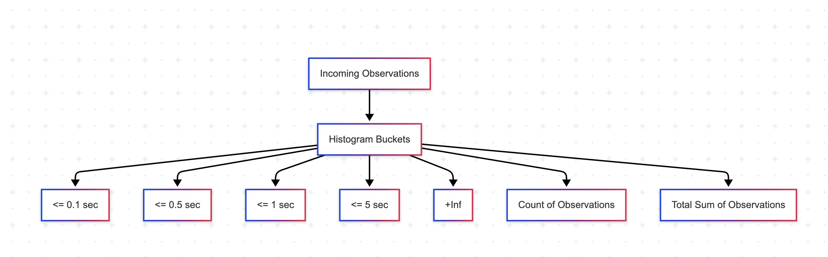
The buckets are inclusive and cumulative. For example:

• <= 0.1
• <= 0.3
• <= 1.0
• <= 5.0
• +Inf: a special bucket that captures everything above the last boundary

Each bucket has a corresponding time series with the suffix _bucket, which Prometheus uses to calculate trends and percentiles.

Querying Histograms with PromQL

To make histograms useful, you typically query their buckets using rate() and aggregate them with sum():

# Bucket-wise request rates over the last 5 minutes
sum(rate(http_request_duration_seconds_bucket[5m])) by (le)

To estimate quantiles like the 95th percentile:

histogram_quantile(0.95, sum(rate(http_request_duration_seconds_bucket[5m])) by (le))

This gives you a statistical approximation of request durations using real-time data across instances.

Histogram Implementation

var requestDuration = prometheus.NewHistogramVec(
    prometheus.HistogramOpts{
        Name:    "request_duration_seconds",
        Help:    "HTTP request duration in seconds",
        Buckets: prometheus.ExponentialBuckets(0.001, 2, 15),
    },
    []string{"method", "endpoint"},
)

func timedHandler(w http.ResponseWriter, r *http.Request) {
    timer := prometheus.NewTimer(requestDuration.WithLabelValues(r.Method, "api"))
    defer timer.ObserveDuration()

    // Process request...
}

When to Use Histograms Instead of Summaries

Histograms have a few key advantages:

• They can be aggregated across multiple instances or label dimensions
• Ideal for service-wide latency thresholds (e.g., “5% of traffic took longer than 500ms”)
• Work well with PromQL and alerting tools

Things to Look Out For

Histograms are powerful, but they come with trade-offs:

• They generate multiple time series per metric, one for each bucket and label combination
• Poorly chosen bucket ranges can reduce visibility or waste resources
• They offer less precision than summaries for individual quantiles

Before instrumenting with a histogram, ask:
Can I define meaningful bucket boundaries? Will I need to aggregate this metric across services?

If the answer to both is yes, histograms are often the better fit for production use.

Summary Metrics

Summaries are used to calculate quantiles, such as the 90th or 95th percentile, directly inside the application before the data reaches Prometheus. Unlike histograms, which estimate quantiles at query time, summaries handle this logic during instrumentation.

When to Use Summaries

Summaries are a good fit when:

• You need accurate, per-instance percentiles
• Aggregation across services or labels isn’t required
• Local response time tracking is more important than cluster-wide trends

Use them for metrics like:

• Latency of a single endpoint
• Duration of internal jobs or background tasks
• In-process performance measurements where precision matters

How Summaries Are Structured

A summary metric comes with two additional time series:

• _count: Total number of observations
• _sum: Sum of all observed values

Each configured quantile becomes its own time series. For example:

http_request_duration_seconds{quantile="0.95"}

This gives you the estimated 95th percentile latency, based on the last N observations in a sliding time window.

Limitations to Be Aware Of

Summaries are not aggregatable across multiple targets. Quantiles don’t combine cleanly, so you can’t compute a meaningful 95th percentile across all your services using summaries alone.

They also come with some overhead:

• More CPU and memory usage due to in-process quantile calculation
• Precision depends on configuration (e.g., window size, error margin)
• Higher risk of duplication if multiple quantiles are defined with high-cardinality labels

When to Choose Summaries vs. Histograms

If you need to compute percentiles across multiple instances, stick with histograms. They work with PromQL functions like histogram_quantile() and can be summed across labels and services.

Summaries are better when local accuracy matters more than global trends, especially for fine-grained measurements on individual services.

Practical Recommendation

You don’t have to pick just one. Many production systems use both:

• Use histograms when you need aggregation across instances, for alerting or global dashboards
• Use summaries when you care about precision within a specific service, endpoint, or job

Choosing the right type depends on what you’re measuring, and how you plan to use the data once it lands in Prometheus.

Built-In Prometheus Alerts for Scale and Stability

Monitoring Prometheus itself is just as important as monitoring your applications. These alerting rules help you catch early signs of overload or misconfiguration.

groups:
  - name: prometheus_performance
    rules:
      - alert: HighCardinality
        expr: prometheus_tsdb_head_series > 5000000
        for: 5m
        labels:
          severity: warning
        annotations:
          summary: "Prometheus cardinality is high ({{ $value }} series)"

      - alert: SlowQueries
        expr: histogram_quantile(0.95, prometheus_engine_query_duration_seconds_bucket) > 5
        for: 2m
        labels:
          severity: critical
        annotations:
          summary: "Prometheus queries are slow (p95: {{ $value }}s)"

HighCardinality

This alert fires when the number of active time series exceeds 5 million for over five minutes. It’s a strong signal that something is generating more series than expected, usually due to unbounded labels, overly granular metrics, or misuse of histograms. If left unchecked, this can slow down ingestion and increase memory pressure.

Start by checking which metrics contribute the most series using:

topk(10, count by (__name__)({}))

Then inspect label sets with:

count by (__name__, label_name)({__name__=~".+"})

SlowQueries

This alert tracks the 95th percentile of internal Prometheus query duration. If queries consistently take longer than 5 seconds (p95), it likely means the server is overloaded or running inefficient queries, especially those involving large aggregations or high-cardinality metrics.

You’ll want to check:

• Active queries in /api/v1/query_exemplars or /api/v1/query_range
• Query logs (if enabled) for slow patterns
• Whether rules or dashboards are sending frequent, heavy queries

Making Metrics Easier to Understand

Prometheus collects the data, but dashboards are where that data becomes usable. Clear visualizations help teams monitor, debug, and make decisions quickly.

Here are a few practical guidelines:

• Use tools that match your scale
  Grafana is widely adopted and works well with Prometheus for most workloads. For larger environments or high-cardinality use cases, Last9, an Otel-native Telemetry Warehouse is purpose-built to handle scale, offering fast queries without needing pre-aggregation or sampling.
• Focus on core signals
  Track latency, traffic, errors, and saturation. Organize views by service or endpoint rather than infrastructure layers, so issues are easier to trace end-to-end.
• Avoid raw metrics
  Graphing totals like counters without using rate() or increase() can mislead. Use time-based functions to surface actual trends.
• Document what you emit
  Define what each custom metric means, what the labels represent, and how they’re intended to be used. Last9 supports metric metadata, so this information is easy to reference directly from dashboards.

Getting started takes just a few minutes and works alongside your existing setup, no changes required.

Metrics exploding?

Counters, gauges, histograms: they all add up. When cardinality grows faster than your memory, Last9’s streaming aggregation keeps queries fast without the OOM crashes.

Try Last9 free →

FAQs

What are the types of metrics in Prometheus?

Prometheus supports four metric types: Counter, Gauge, Histogram, and Summary. Each type offers distinct capabilities for tracking different system behaviors.

What are the metrics of Prometheus scale?

Prometheus scales by scraping time series data based on a label-rich model. Its scalability depends heavily on cardinality, the number of unique label combinations. Histograms with too many histogram buckets or highly dynamic labels can strain a Prometheus deployment.

What metrics does Prometheus monitor?

Prometheus can monitor any metric your API, service, or infrastructure exposes through supported client libraries. Common examples include CPU usage, memory consumption, API response times, Kubernetes pod states, and business events like total HTTP requests or transactions.

What is the format of Prometheus metrics?

Prometheus metrics use a plaintext exposition format served over HTTP. Each line includes a metric name, an optional label set, and a value. Example: http_requests_total{method="GET", code="200"} 1027

What are Prometheus metrics?

Prometheus metrics are structured time series built on a flexible data model. Each metric includes a name, labels, a sample value, and a timestamp. Samples are collected at intervals and queried using PromQL.

What are some use cases for gauges?

• Memory usage in Kubernetes containers
• Number of API connections or sessions
• Queue length or disk space remaining

Gauges are ideal for system values that fluctuate over time.

When to use histograms?

Use a histogram when you need to analyze value distributions or percentiles, such as:

• API response times bucketed into latency ranges
• The total sum and count of observations over time
• Configurable buckets that help track thresholds (e.g., 99th percentile)

What would be the ideal metric type for that job?

• Counting events or HTTP requests: Counter
• Monitoring real-time resource usage: Gauge
• Tracking response times across ranges: Histogram
• Getting client-side quantiles like the 99th percentile: Summary

Why use Summary metrics?

Summary metrics are computed on the client side. They are ideal when you want accurate percentiles, like 99th percentile latency, on a per-instance basis. Use them when aggregation is not needed but high-resolution insight is.

How do you create custom metrics in Prometheus?

Use Prometheus client libraries (Go, Python, Java, and others) to define and expose metrics from your service. Prometheus then scrapes them for analysis, alerting, and dashboards. Add labels thoughtfully to avoid high cardinality.

How does the Prometheus counter metric type work?

A counter increases monotonically. It tracks events like API hits, background job runs, or errors. When the process restarts, the counter resets, but functions like rate() account for the reset.

How do Counter metrics work in Prometheus?

Counter metrics represent a running total of event occurrences. Prometheus scrapes the value at regular intervals, and PromQL can compute the rate of change or increase over time, even across counter resets.

How do you define a new metric type in Prometheus?

You cannot define new metric types beyond the standard four. You can define custom metrics using the existing types through client libraries, setting up counters, gauges, histograms (with configurable buckets), or summaries for your needs.

What are Prometheus metric naming conventions?

Prometheus metric names should use snake_case, start with a single-word application or domain prefix (for example http_ or node_), and end with the unit of measurement (for example _seconds or _bytes). Counters add a _total suffix, such as http_requests_total. Keep names descriptive but stable, and put anything that varies into labels rather than the metric name.

How do you reduce high cardinality in Prometheus metrics?

Cardinality is the number of unique label-value combinations per metric. To keep it under control, never put unbounded values like user IDs, request IDs, full URLs, or timestamps into labels. Normalize free-form values into a small fixed set (for example, map raw error strings to an error_type label). Drop unneeded labels at scrape time with metric_relabel_configs, and pre-aggregate expensive label sets using recording rules. For finding the worst offenders, see how to manage high cardinality metrics in Prometheus.

What do the _sum, _count, and _bucket suffixes mean?

Histograms and summaries expose more than one time series. The _count series is the total number of observations, and _sum is the total of all observed values, so _sum / _count gives the average. Histograms additionally expose a _bucket series per bucket boundary, labeled with le (less than or equal), which histogram_quantile() uses to estimate percentiles.