How Streaming Aggregation Works

In our earlier pieces, we explored how rich telemetry pays off — faster incident resolution, stronger SLAs, and a clearer view of system behavior. But as telemetry volume grows, the challenge becomes making that richness affordable and queryable at scale.

Streaming aggregation helps you do exactly that. By moving heavy aggregation work from query time to ingestion time, you keep the same depth of insight while making dashboards faster, queries lighter, and storage more efficient.

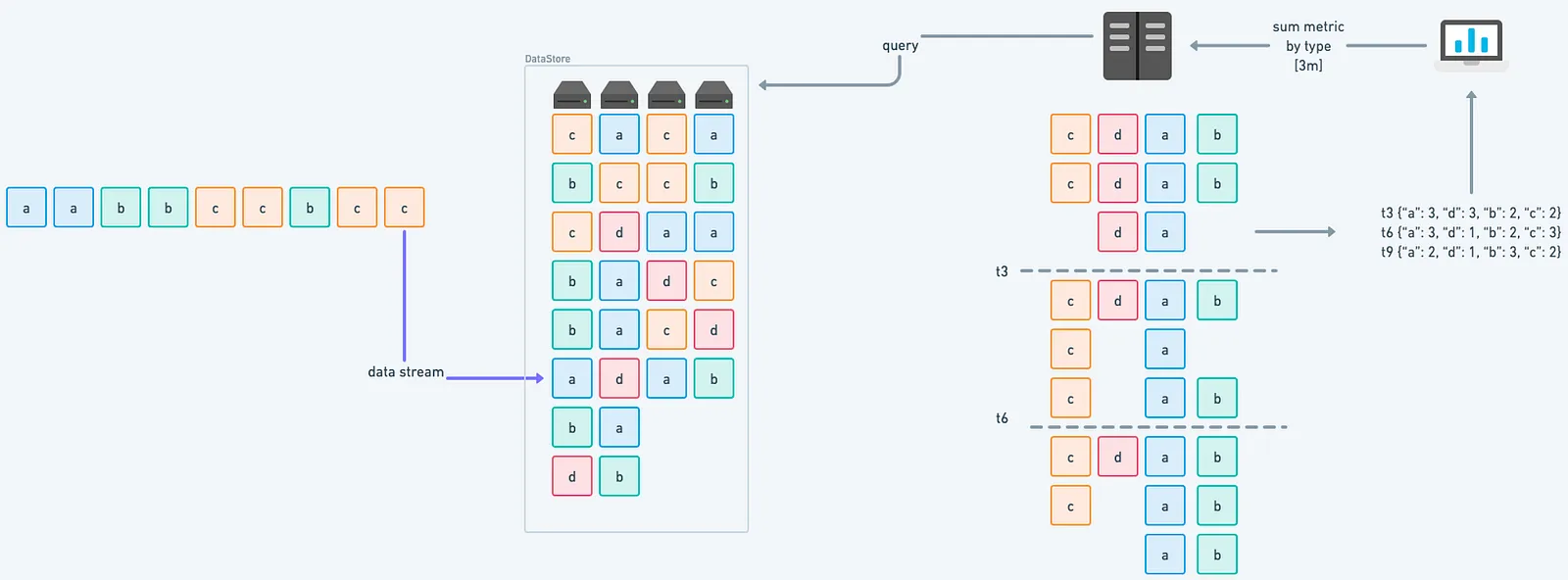
How Traditional Querying Slows Down Your Dashboards

Ordinarily, as metrics arrive, they’re written as-is to your time series database. When you run a query like:

sum by (type) (metric_name{}[3m])

Here’s what happens behind the scenes:

• All matching samples are pulled from storage
• They’re grouped by timestamp and label combinations
• Aggregation logic runs across the entire dataset — every single time

This process repeats with every dashboard refresh. And as your data volume grows, so does the cost of doing this over and over — millions of time series scanned just to render a single panel.

What Changes When You Enable Streaming Aggregation

Streaming aggregation changes when and how your system processes metrics. Rather than reactively crunching numbers at query time, you define what matters early, closer to ingestion.

That doesn’t mean throwing away detail. It means structuring your metrics to reflect how your team thinks about problems.

Here’s what that could look like:

• Skip labels like hostname, instance, or pod when you don’t need per-host granularity
• Precompute PromQL-heavy constructs—like histogram quantiles or error rates
• Build focused aggregates like:

sum without (instance, pod) (grpc_client_handling_seconds_bucket{})

The result:

• Faster dashboards — with fewer surprises during high load
• Lower compute and storage — without compromising on visibility
• More meaningful metrics — shaped to your team’s use cases and workflows

High cardinality gives you the raw material—streaming aggregation helps you shape it into something useful.

Where Streaming Aggregation Fits

Streaming aggregation sits between your collectors and your time series database, transforming metrics before they’re stored.

This approach doesn’t require changes to your application instrumentation, and your dashboards and alerts continue to work the same way—they just query a dataset that’s already been shaped for speed and efficiency.

Here’s how it fits into a typical flow:

1. Applications emit metrics — Your services, containers, or jobs expose metrics in the usual way.

2. Collectors gather data — Prometheus scrapes endpoints, or OpenTelemetry agents receive/export metrics.

3. Streaming Aggregation Layer processes metrics — This is where your rules run:

   • Compute aggregates like percentiles, sums, or counts.
   • Remove labels you don’t need, reducing series count.
   • Precompute expensive PromQL expressions.

4. Time Series Database stores results — Only the aggregated, high-value metrics are written to storage.

5. Dashboards and alerts query faster — Grafana panels and alert rules work exactly as before, but with fewer, lighter series to process.

Different deployment patterns make streaming aggregation flexible:

• Edge aggregation — Runs as a sidecar next to each Prometheus instance or OpenTelemetry collector. It processes metrics right where they’re collected, which means you cut down the volume before it leaves the node or region. This works well for distributed clusters where local processing avoids pushing huge datasets over the network.

• Centralized aggregation — All metrics from multiple collectors feed into a single aggregation tier before reaching the global time series database. This is handy when you need organisation-wide metrics, like total API latency across all regions, and want to manage aggregation rules in one place.

• Hybrid — A mix of both approaches. High-volume, noisy metrics are aggregated at the edge to reduce transfer load, while multi-cluster or cross-region summaries are computed centrally. This model fits large infrastructures where you need both local efficiency and global visibility.

Why Not Just Use Recording Rules?

Recording rules are a useful way to precompute queries, but they run after data is already ingested. That means you’ve still stored the raw, high-cardinality time series — and paid the cost of collecting and retaining them.

Streaming aggregation works earlier in the pipeline. It handles metrics as they arrive, so you can shape data at the source and skip writing unnecessary series altogether.

You can still use recording rules for longer-term summaries or business-level rollups. But if your goal is to reduce ingestion load, speed up queries, and keep your storage lean, streaming aggregation gets you there first.

When Streaming Aggregation Becomes Critical

You introduce streaming aggregation when your metrics system starts showing signs of strain or when future growth makes it inevitable. The tipping point varies by organisation, but the progression follows common patterns.

Early Stage – Set Guardrails Before Growth Hits

You might be handling dozens of services, standard scrape intervals, and most queries return under a couple of seconds. Things are smooth, but the risk comes from adding labels:

• Example: A request latency metric tagged with le, handler, and hostname produces ~90,000 unique series.
• By dropping the hostname label during streaming aggregation, this drops to ~900 series—a 100× reduction, while keeping service-level visibility.

Starting aggregation early sets smart defaults, so when metrics start scaling up, you’re already ahead of the curve.

Growth Phase – Watch Your Storage and Latency

At this point, business labels like customer_id, user_id, or transaction_id creep in, and suddenly your series count balloons. You start feeling the pinch:

• Storage costs climb faster than expected.
• Wide dashboards time out.
• Engineering teams restrict time ranges just to keep dashboards usable.

Streaming aggregation here slims down metrics at ingestion, keeping only the parts you need and avoiding storage bloat.

Enterprise Scale – Queries Stall Under Pressure

Now you’re in the hundreds of millions of series range. Incident response becomes a game of patience:

• Complex dashboards involving histograms or high-cardinality metrics take minutes or fail outright.
• Your visualization tools start to break under load.

This mirrors what Prometheus tackled with remote read streaming:

• Before: querying 10K series over 8 hours took ~34.7 seconds.
• After: it dropped to ~8.2 seconds, a 4× speed improvement.

Streaming aggregation achieves the same principle, preparing data smarter, serving it faster.

Platform Scale – You Can’t Operate Without It

At a global scale, thousands of services across regions, you’re dealing with an extremely rich telemetry set:

• Millions of metric series covering both infrastructure and business dimensions
• Multi-service dashboards pulling data from multiple regions
• Large-scale retention requirements for historical analysis

Streaming aggregation helps make this data workable in real time by:

• Producing service-level or region-level aggregates alongside the full detail
• Reducing the amount of data that needs to be processed per query
• Ensuring dashboards and alerts respond within operational timeframes

This way, you retain the depth and granularity of your telemetry, while making it practical to explore and use under heavy load.

Time-Based Aggregation: Tumbling vs. Sliding Windows

Streaming aggregation uses time windows to group metrics as they arrive. The two most common strategies are:

• Tumbling windows: Fixed, non-overlapping intervals.
  Ideal when you want to group metrics into clean chunks—like “requests per minute.”
  Example: Group metrics into 1-minute buckets — 0:00 to 0:01, 0:01 to 0:02, etc.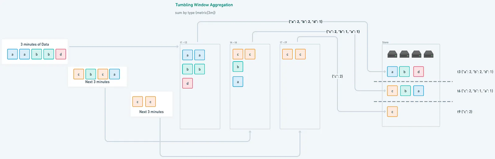

  

• Sliding windows: Overlapping intervals that move forward continuously.
  Useful for smoothing out data or triggering alerts based on rolling averages.
  Example: Calculate a rolling average every 10 seconds over the past 1 minute.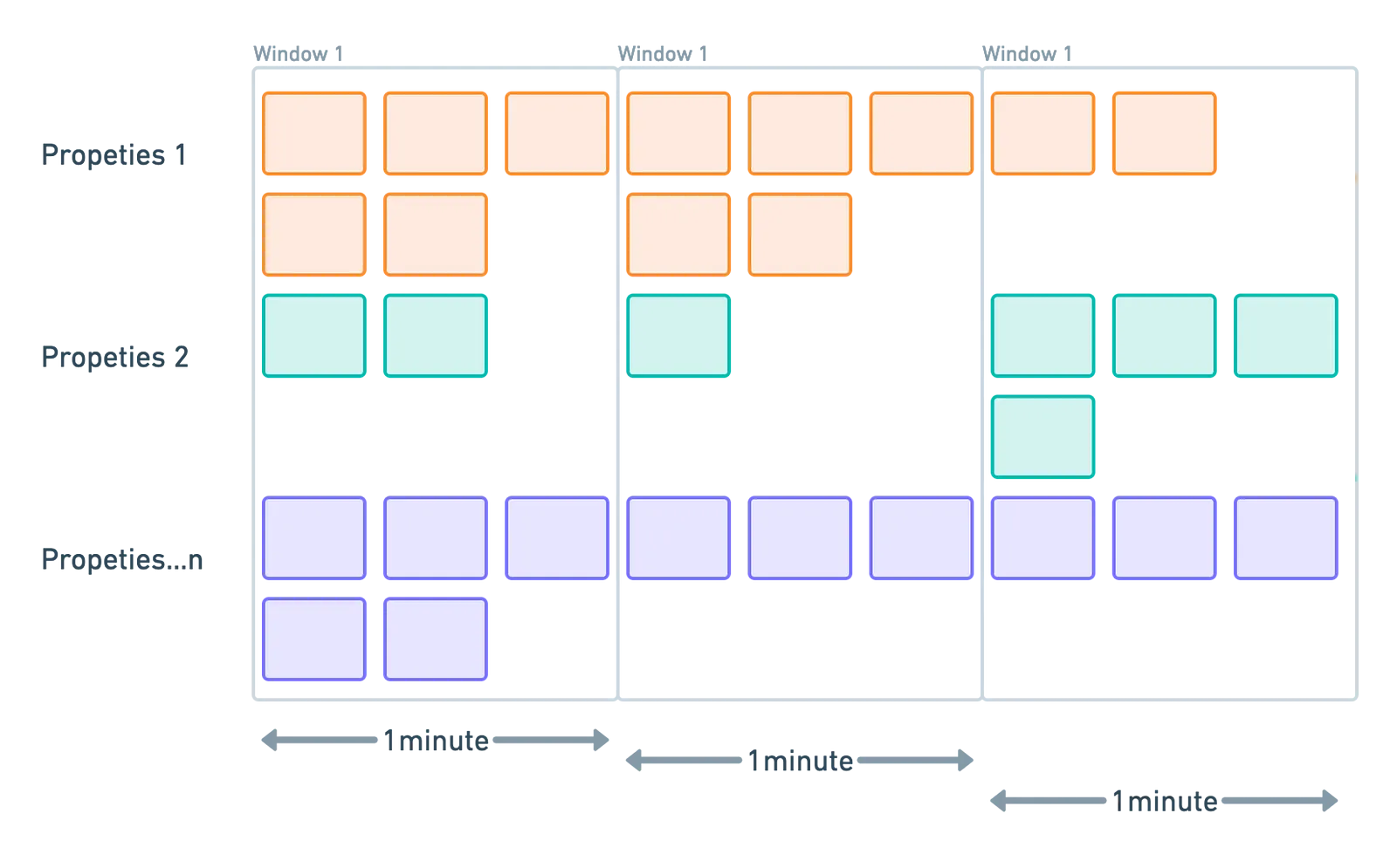

  

With recording rules, aggregation happens after metrics are already stored—so time windows are applied post-ingestion. In contrast, streaming aggregation applies windowing as metrics arrive. This means your window strategy directly shapes what gets stored and how queries perform.

Time windows define when metrics are grouped. For simple counters or gauges, that’s enough. But for histograms, you also need to coordinate how they’re grouped. All parts of a histogram — _bucket, _sum, and _count — must use the same window boundaries to keep your percentiles and averages accurate.

How Histograms Work in Streaming Aggregation

Histograms represent distributions over time, not just single values. And when using streaming aggregation, you need to be deliberate in how you handle them.

Each histogram metric consists of three related time series:

• <metric>_bucket – counts for each latency bucket
• <metric>_sum – total sum of all values
• <metric>_count – total number of observations

To maintain accuracy, all three need to be aggregated together during ingestion. Dropping a label or changing a window on just one of them will throw off queries that rely on a complete view of the distribution.

Let’s say you’re aggregating request latency metrics across all instances:

sum without (instance) (http_request_duration_seconds_bucket{})

sum without (instance) (http_request_duration_seconds_sum{})

sum without (instance) (http_request_duration_seconds_count{})

This keeps the histogram shape intact, so your downstream queries for averages, P95s, or traffic volumes stay correct, without needing reprocessing at query time.

Key Streaming Aggregation Techniques for Cardinality Control

Streaming aggregation offers three practical approaches to structuring high-cardinality metrics:

1. Label Dropping: Removing Unnecessary Detail

Not every label adds meaningful value. Some dimensions, like unique IDs or highly dynamic paths, create huge amounts of series, but rarely help with debugging or alerting.

Streaming aggregation lets you drop these labels at ingest, before they inflate your storage or slow down queries.

Original metric:

http_request_duration_seconds{service="payment", path="/api/v1/transactions/123456", user_id="u-89273", instance="pod-8371"}

After dropping unnecessary labels:

http_request_duration_seconds{service="payment", path="/api/v1/transactions", instance="pod-8371"}

Here, we’ve kept the parts that help answer “is this endpoint slow?” and removed the parts that don’t move the needle for observability. The result? Same business signal—fewer distractions.

2. Label Transformation: Preserving Meaning Without Overload

Sometimes, you do want to keep user or business context — but not at full granularity. That’s where label transformation helps.

Streaming aggregation allows you to group raw values into broader categories in real time, preserving the signal while avoiding unnecessary churn.

Original metric:

api_request_count{customer="acme-corp", endpoint="/users/12345/profile", region="us-west-2a"}

After transformation:

api_request_count{customer_tier="enterprise", endpoint_type="user_profile", region="us-west-2"}

This way, you can still answer questions like:

• Are enterprise customers seeing more errors?
• How are user profile endpoints performing across regions?

You keep the insight. You just don’t pay the cost of tracking every user and every path variation individually.

3. Pre-Aggregation: Creating Statistical Summaries Across Dimensions

One of the most effective ways to work with high-cardinality metrics is to pre-aggregate them across the dimensions you care about, right at ingestion.

Original metric (millions of time series):

request_duration_seconds{service="auth", endpoint="/verify", user_id="u-12345", region="us-east-1"}

After pre-aggregation (just a few time series):

request_duration_seconds_avg{service="auth", endpoint="/verify", region="us-east-1"}

request_duration_seconds_p95{service="auth", endpoint="/verify", region="us-east-1"}

request_duration_seconds_count{service="auth", endpoint="/verify", region="us-east-1"}

By computing summaries like average, p95, and count at ingest, you avoid storing user-level detail while still capturing latency trends and volume across key dimensions like service, endpoint, and region.

This approach is especially useful for dashboards and alerts that don’t require full granularity but still need fast, meaningful insights.

Common Pitfalls with Streaming Aggregation and How to Avoid Them

Even experienced teams can run into issues when implementing streaming aggregation. Here are a few common ones — and how to avoid them.

Pitfall 1: Overly Aggressive Aggregation

If you aggressively drop high-cardinality labels (like user_id or instance) during streaming aggregation, you lose the ability to drill down during incidents. You’ll know something is wrong — but not who it affects or where it’s happening.

How to avoid it:
Keep a limited window of raw metrics—either:

• For a short recent time range (e.g., last 10–15 minutes), or
• For a sample of traffic (e.g., 1–5% of requests)

This gives you enough granularity for on-demand investigation, without storing everything at full fidelity.

To go further, you can also set up a fallback.

• Under normal conditions, you aggregate as usual.
• But if error rates or latency cross a threshold, you temporarily bypass aggregation for specific services or labels, so raw data is preserved in real time for debugging.

This keeps your system efficient day to day, but still gives you the detail you need when things break.

Pitfall 2: Stale Aggregation Rules

Aggregation rules that worked well initially can quickly become outdated as your system evolves. Sticking to static rules risks missing new or shifting high-cardinality dimensions, leading to blind spots in your monitoring.

High cardinality provides rich, detailed insights, but only if your aggregation rules evolve alongside your data.

How to avoid it:
Regularly review and update your aggregation rules. Use alerts or monitoring tools to detect emerging cardinality dimensions early, so you can adjust aggregation before problems grow.

Pitfall 3: Confusing Metric Naming

When you have multiple versions of a metric, like raw, averaged, and percentile values, it’s easy to lose track of what each one means. Teams often end up asking: Which one should I query? or worse, they pick the wrong one during an incident.

How to avoid it:
Adopt a clear, consistent naming convention that makes the metric’s purpose obvious at a glance.

For example:
Instead of this:

http_request_duration_seconds

http_request_duration_seconds_1

http_request_duration_seconds_2

Use something like:

http_request_duration_seconds_raw --unaggregated

http_request_duration_seconds_avg -- average latency

http_request_duration_seconds_p95 -- 95th percentile latency

http_request_duration_seconds_count -- total number of requests

When naming reflects meaning, onboarding gets easier, debugging gets faster, and nobody has to guess what a metric is showing—especially during incidents.

Pitfall 4: Resource Constraints

Streaming aggregation is compute-intensive. As the number of metrics and labels grows, real-time processing can put pressure on your collectors or ingestion pipeline, leading to slowdowns, dropped data, or increased lag.

How to avoid it:
Keep an eye on CPU usage, memory consumption, and processing latency. If aggregation begins to impact performance, consider:

• Scaling horizontally — run multiple collector instances
• Splitting responsibilities — handle ingestion and aggregation in separate stages
• Using dedicated components — offload heavy computations to a standalone service or sidecar

Example:
If your collector is responsible for both scraping and aggregating, it’s more likely to hit resource limits under load. Moving aggregation to a separate service can help maintain reliability without sacrificing detail.

How Last9 Helps You Work with High Cardinality

High-cardinality metrics carry valuable detail, but without structure, they can be expensive to store and slow to query.

With Last9’s PromQL-based Streaming Aggregation, you can define rules to drop labels, transform dimensions, and generate new metrics, right at ingest. No changes needed to your application code or configuration.

This lets you stay ahead of cardinality limits while keeping your metrics usable and lightweight.

Up next: We’ll look into high cardinality data patterns, hidden correlations in dimensional metrics, cloud-native cardinality explosion mechanics, and when and why traditional metrics fail.