How we tame High Cardinality by Sharding a stream

Levitate is Last9’s Time Series Data Warehouse. One of Levitate’s biggest propositions is its commitment to resolving high-cardinality workflows and needs. This post is part of a series of articles on the steps necessary to create high-performance data systems.

This particular article focuses on solving extreme cardinality in TSDBs with Sharding, without incurring performance penalties.

High performance is like glass — it can be made extremely effective, but it remains fragile. Similarly, building a high-performance system that lacks Reliability is like constructing a house of cards. It may seem impressive, but it is easy to collapse.

So, how can you develop something that delivers consistent, high performance at scale? One word — Sharding!

Don’t just take our word for it - hear from the experts themselves.

Part 1 of this series (What goes into a Gateway) discussed the construction of a high-performance and scalable gateway that addresses the problem of high cardinality.

Preface

To ensure efficient data storage, Gateways communicate with receivers that distribute the data evenly across Storage nodes before it is stored. There are two downstream modes for this data:

• Direct writes to the storage
• Optionally, extremely high cardinality data can be sent to Streaming Aggregators, which provide an almost 100x cardinality boost. This can be particularly useful in cases where the data is complex and requires additional processing power to be processed effectively. For more information about Streaming Aggregations, see 🚿 Streaming Aggregation.

Before proceeding, it’s important to distinguish between two problems that can arise in high-cardinality workflows.

• The first is high performance, which focuses on optimizing the speed and efficiency of data processing.
• The second is high availability, which ensures that data is always available and accessible to users.

High Availability

Replication

Replication is a technique that makes exact copies of the data and stores them across different hosts. Database designers use long-used replication as a way to design fault-tolerant systems. When one of the hosts fails, other replicas remain operational.

One easy way out is to Spray the data across the cluster and have all nodes respond with null or actual response.

This is something VictoriaMetrics does 👇

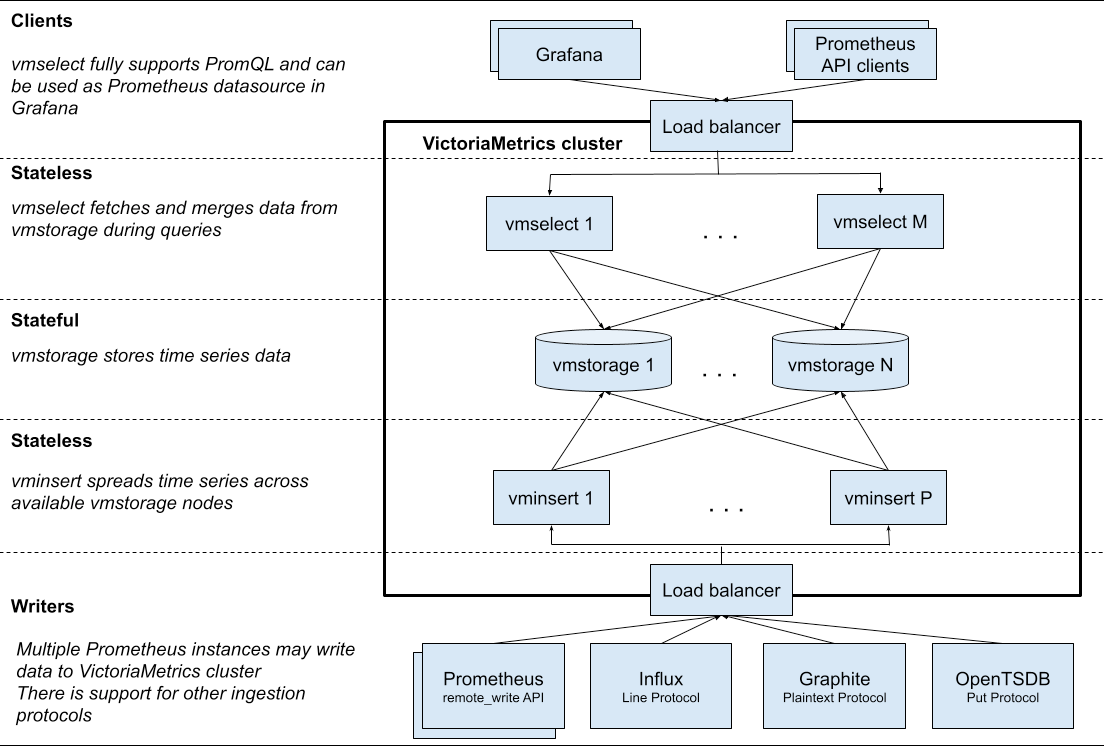
And so do other peers like m3DB.

Spray and Wait

Once the data is spread across replicas, a new set of challenges emerges:

• You can either spread the data across every single replica
• In such a case, how do you allow for partial failures? Is one write enough, or do you need N writes?
• Waiting for N-acknowledgements can make a system really really sluggish. And, in turn, it doesn’t solve the Performance requirements.
• When you have M out of N sufficient criteria, how does a system identify which node has the data and which doesn’t?

This approach is called “Spray the data and Wait”. The roots of this technique can be traced back to this approach, but it is grossly inefficient.

With replication, we can successfully solve the data availability problem, which often leaves us with compromised system performance. This type of problem requires additional techniques of horizontal scaling, which are discussed below.

High Performance

Additionally, replicating such massive compute boxes multiplies the entire cost by the N-replication factor, achieving the reverse of what Streaming aggregations can do: deliver knowledge across large datasets at a fraction of the cost.

Imagine this Pictorially:

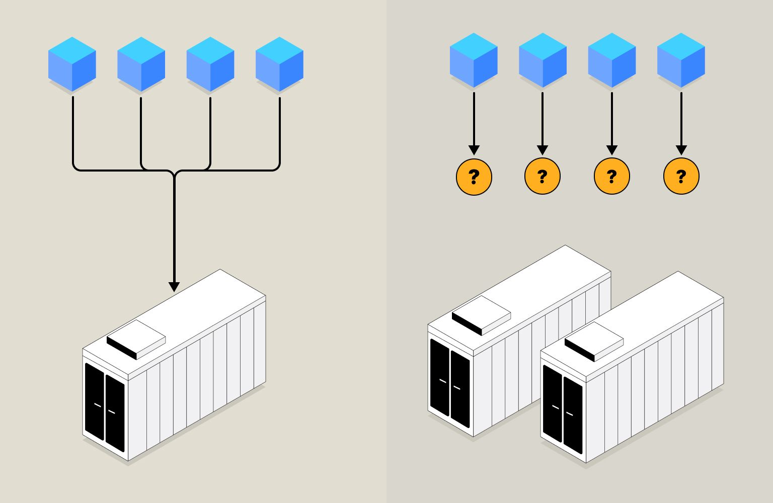
Multiple gateways can send data to a single receiver, which can become a single point of failure. To overcome this issue, it is important to scale out the receivers of data horizontally. However, this raises the challenge of how to decide on the strategy for sending this data.

Multiple options come to mind:

• Load Balancing across receivers.
• Sharding.

Sharding vs. Load Balancing

💡 It’s important to remember that sharding doesn’t replicate data. Only one receiver gets the data. This detail is sometimes overlooked and can cause problems later on. I’ve seen experienced designers miss this and have to redo their sharding technique. They assumed they could access data across shards, but that wasn’t the case.

Load balancing involves simply routing subsequent requests to balance the load. Sharding, however, goes a step further by assigning unique identities and addresses to distinct chunks of data.

This approach is based on developing an efficient address scheme for data at rest. This enables the system to locate and retrieve the required data predictably. By implementing sharding, the system can distribute the data across multiple servers, thereby enhancing the system’s scalability and reliability. Moreover, the sharding approach can help minimize the impact of system failures by ensuring that the failure of any single server does not lead to the loss of the whole dataset.

See the following visual representation for a better understanding:

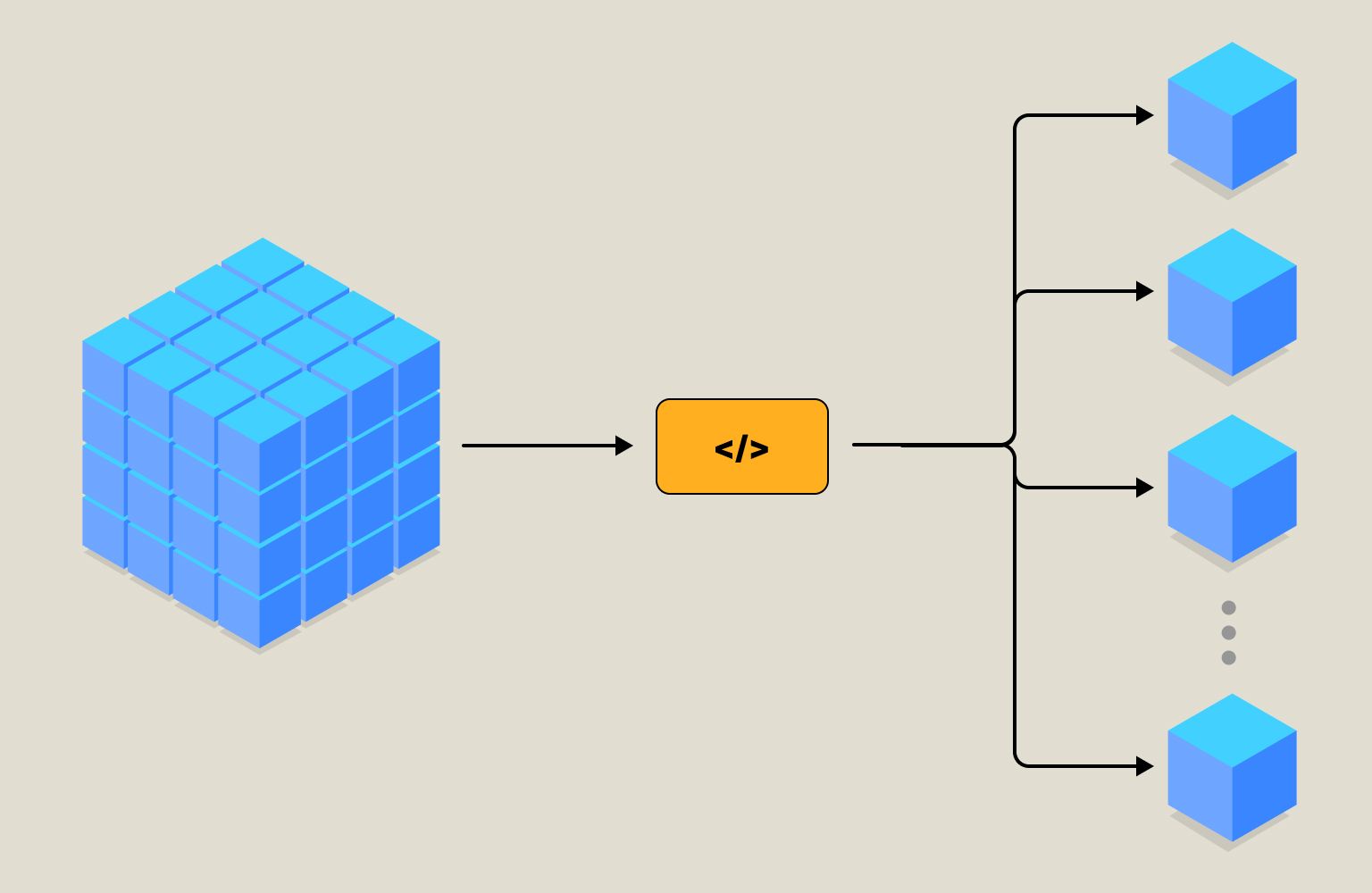
Each Chunk is designed to know its specific location within the larger system. This includes not only its physical placement but also its functional relationship to other Chunks and the system as a whole. For example, Chunks could be divided based on the frequency of access, physical separation across departments, or even user_id. Whatever the method, the goal is to maintain a separate locality.

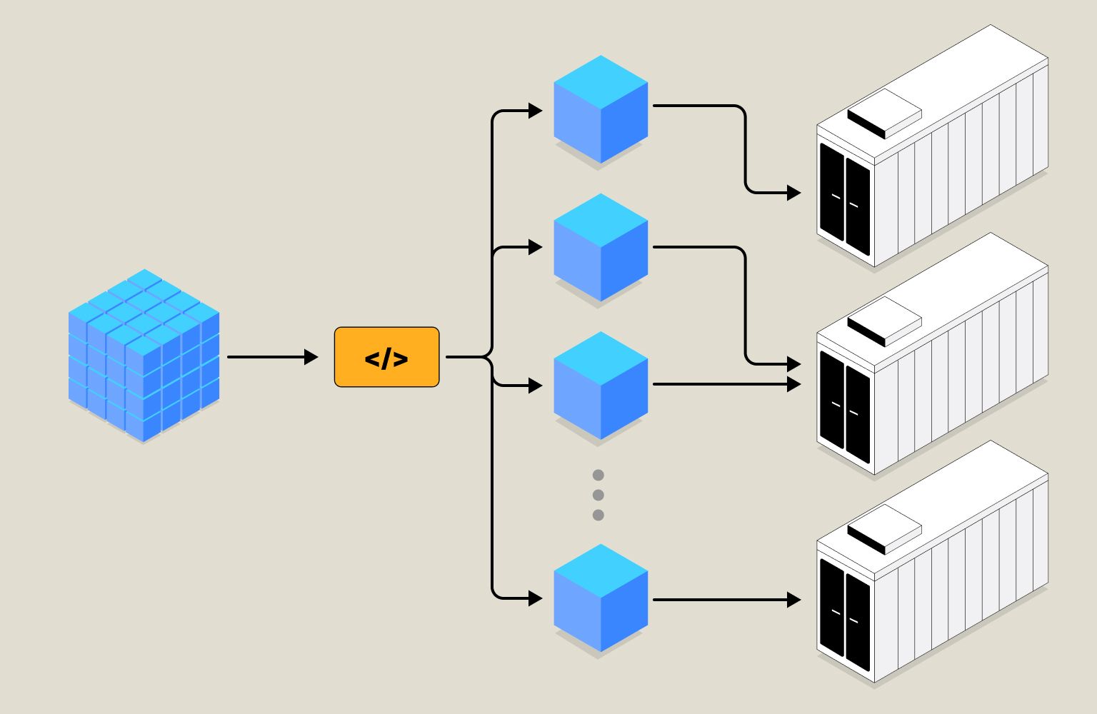
Splitting the Data

Before deciding where data must be sent, there is an additional step of splitting the data that is crucial for the effective functioning of a data storage system.

• Based on a Range of Values

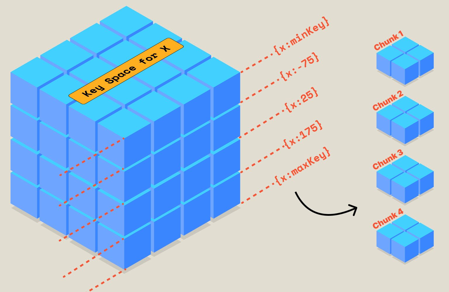
In this technique, chunking is based on the range of values suitable for the available or planned number of shards. Here’s a visual representation: based on the value of x, we divide the data into four chunks. This technique is simple and repeatable. However, if you query overlapping ranges of x, it requires a query and joins across multiple shards, ruling out the possibility of leveraging data-locality-based processing closer to the chunk.

• Based on a Key in the Data
  In this technique, Chunking is dynamically assigned using a formula. The simplest example would be:

This hashing technique does not require pre-knowledge of the Data distribution, allowing data to be randomly distributed. However, because of that, it can create data skews. i.e., More keys may end up in the same chunk number. Such skewed shards are also called Hot Shards.

Data Locality

One key factor to consider when it comes to sharing data is Data Locality. This refers to the concept that data is often accessed more frequently by processing units that are physically closer to it, rather than units that are located farther away. This can have a significant impact on the accuracy of the operations that are performed on the Data. Let’s explain that again with more context of Streaming Aggregations.

The goal of Streaming Aggregation is to collect a continuous flow of samples (which can be in the millions per minute) and apply a function to this data to produce a single value.

There are two parts to this problem:

• Collecting and storing data across Shards to increase throughput and reliability
• The Compute layer reads the sharded data and applies an in-memory function

If, during the function, data has to be obtained from a non-local instance, it will result in:

• Inaccuracy
  Either you don’t retrieve non-local data and suffer from the Fallacies of Distributed Computing.
• Performance reduction
  If you have handled the Fallacies, the network comes at a cost. Remember, reading from RAM is faster than reading from a disk, which is faster than reading from a network.

Therefore, it’s crucial to have all the data required for the function to be in the same place as the function. This cannot be achieved dynamically, but rather by selecting a key based on knowledge of the data. For example, in the case of streaming aggregation like avg_user_session, you will normally use a key like user_id.

💡 The problem doesn’t stop here. If you run multiple functions on the same data, ALL of them must find the data that is local to them to run accurately and efficiently. Remember, there are NO duplicates created for the data. This makes choosing the sharding key all the more important.

We noticed that this eventually becomes a query-independent key that closely represents the sharding pattern in the application infrastructure.

Repeatable Hashing

Another important consideration is the repeatability of hashing. To ensure data locality, it is crucial that the shards remain the same as they were during the initial hashing. Any changes to the hashing logic due to restarts or infrastructure changes should not result in different outputs.

For example, let’s say we aggregate avg_user_session and use the user_id as the shard key. We have two shards, and we use a simple modulo function to distribute the data: user_id % num_shards.

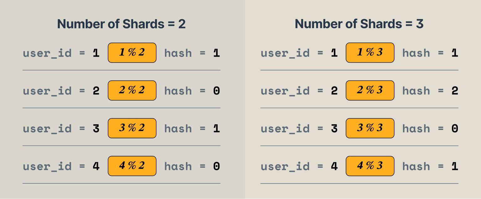
Here is a visual illustration that will help you better:

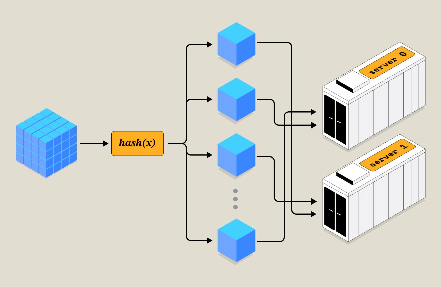
Stateful Hash Tables

To solve this problem, we need to keep track of the assigned hash for each key in a hash_table. When we add a new node to the infrastructure, it only affects new arriving keys. This is a practical design advantage because we can add more resources as needed to handle any “extra/unexpected” load, without affecting the existing load/spread.

💡 Once again, we must pay attention to the right choice of the hashing key. This is explained below.

Suppose we hash on transaction_id and decide to save that in the hash_table. The size of the transaction_id hash table would increase exponentially, which is a fragile decision. In case of extreme load, where hashing is expected to benefit performance, the existing lookup of known keys will keep getting slower. You would be forced to solve for fast indexes and optimize the hash_table storage problem. This is a pursuit that can be avoided by choosing the right hash_key that is anti-fragile OR reaps higher rewards as the scale increases. Since the number of shards is limited, a good hash_key + hash_function that can map an exponentially large set to only 5 values can be used without difficulty.

Challenges with Sharding

One of the main issues with sharding is the increased complexity it brings to the database architecture. When data is partitioned across multiple nodes, it becomes harder to maintain consistency and ensure data integrity. Additionally, sharding can lead to performance degradation if not done properly. This is because queries that require data from multiple shards may take longer to execute, which can impact the overall system performance.

Another challenge with sharding is that it requires careful planning and coordination to ensure that the data is properly distributed across the shards. This involves deciding on the sharding key, which determines how data will be partitioned, and ensuring that the data distribution is balanced across the shards to avoid hotspots.

Finally, sharding can also introduce new failure scenarios, such as network partitions or node failures, which need to be handled correctly to avoid data loss or corruption.

Overall, while sharding can provide significant benefits in terms of scalability and fault tolerance, it requires careful consideration and planning.

Choosing the Right Hashing Key

Choosing the right hashing key is of paramount importance, as it is the main address scheme. While a database system cannot pick the most optimal sharding key on its own, which is perfectly balanced, it has to rely on using some sane defaults designed to provide guaranteed isolation and fault tolerance. Additionally, piggybacking on user input can help even out the balancing of data. Here is an explanation of the techniques.

Sane defaults

We have emphasized enough the importance of the hash_key to make sure all of the following criteria are met

• Data Locality is Preserved
• Hashing is repeatable
• The size of the Hash table is optimally small.

For Levitate, Last9’s managed Timeseries Data Warehouse, a composite key of cluster and metric_name are the default choice of sharding. This allows

• Ensuring that clusters are relatively immune against each other’s failures.
• Not all metrics go down for a cluster if a shard goes down.
• Since cross-metric aggregates are not supported, all data for a metric for a cluster remains local to an aggregator.
• This significantly improves the uptime and avoids blackouts.

User Input

This requires intrinsic knowledge of the data and cannot be done automatically by a system. What may look small today, can grow as the usage grows and the constant balancing and repartitioning is engineering that can be avoided by offloading the decision to one know who knows their data.

We also provide an additional label per metric to be used as a sharding key, in addition to cluster and metric_name.

Choosing the right shard_label can massively boost the reliability and performance of streaming aggregates.

Operational Challenges

Data Hotspots

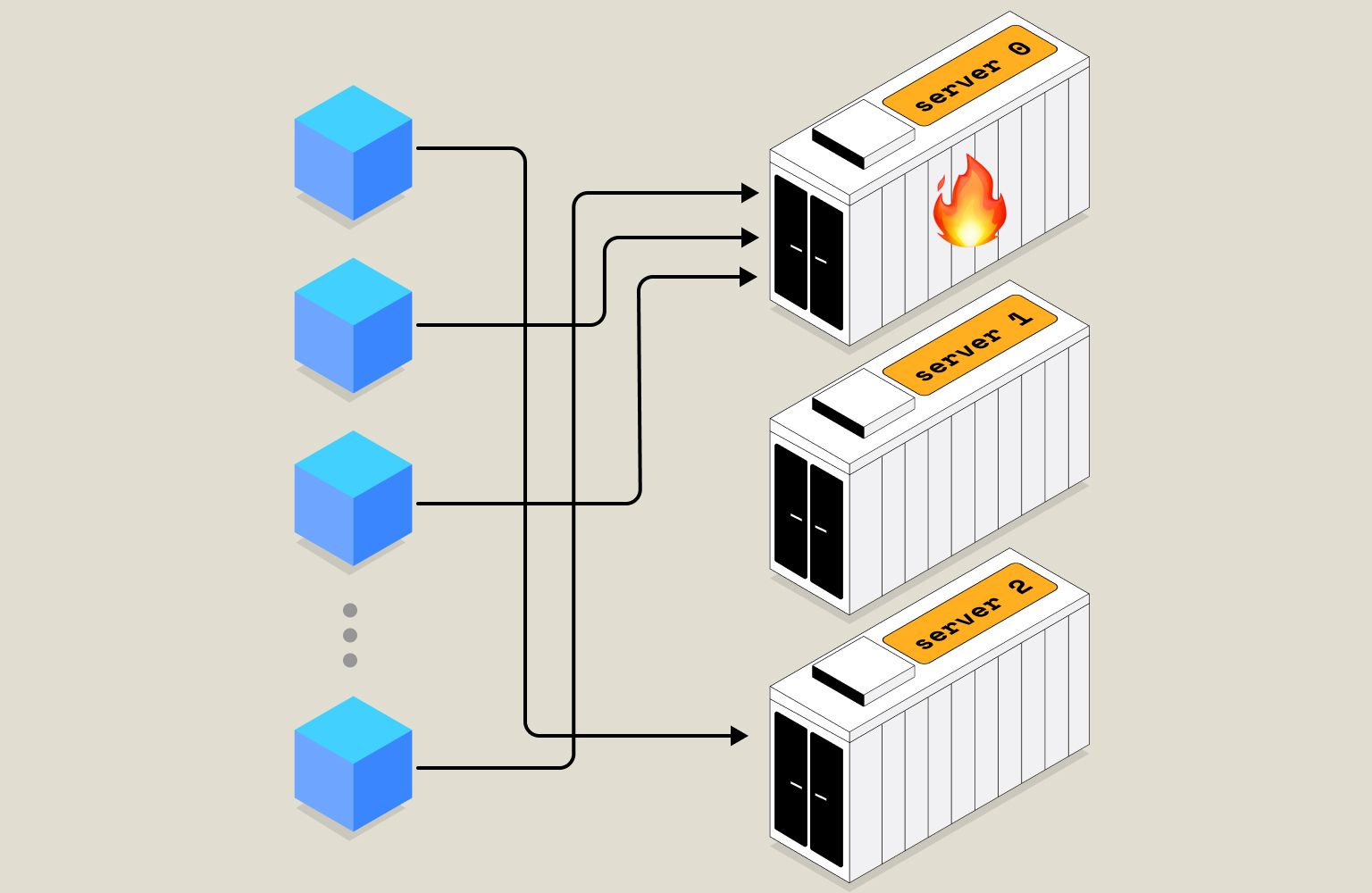
Sometimes, shards may become unbalanced due to uneven data distribution. This can occur when there is a disproportionate amount of data in one physical shard compared to others. For instance, a single physical shard containing customer names beginning with “A” may receive more data than others. This can lead to higher resource usage for that particular shard, which may impact system performance and lead to slower processing times. It is important to monitor shard balance regularly and take steps to rebalance them as needed to ensure optimal performance and efficient resource usage across the entire system.

Adding or Removing Shards

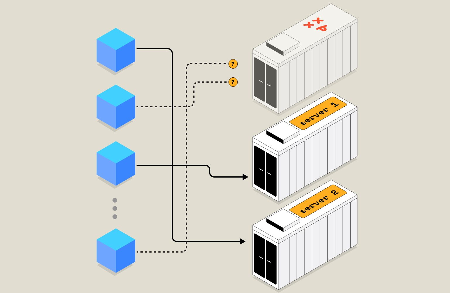
When adding or removing shards, a few operational challenges must be considered, for instance, if a shard is removed, the data must be rebalanced across the remaining shards to ensure they are evenly distributed. On the other hand, adding a new shard can lead to data hotspots and uneven distribution, which can impact system performance. This requires constant monitoring of shards to take appropriate action to ensure optimal performance and efficient resource usage.

Levitate is dedicated to solving high-cardinality workflows and needs. Sharding allows Levitate to scale cardinality needs to unprecedented limits without incurring performance penalties. This means you can now handle larger datasets than ever without worrying about compromising the performance of your system. Our team has worked tirelessly to wrap up the technical challenges behind this feature so you can enjoy the benefits of a simple URL to read and write from.